The Feynman experience · Part 1

The law of large numbers

evergreen · Jan 4, 2019

Introduction

Everyone who studies probability runs into at least two limit theorems: the law of large numbers and the central limit theorem. The law of large numbers describes the result of performing the same experiment a large number of times. It is pervasive in probability and shows up everywhere from gambling to risk management.

Examples

Let’s simulate the two usual suspects of any probability example: a coin and a die.

Coin toss

Let’s track the frequency of heads over 1,000 coin tosses. As throughout this series, we work from scratch in plain Python with NumPy:

import numpy as np

np.random.seed(51)

# 1,000 coin tosses, each 0 (tails) or 1 (heads)
coin = np.random.randint(0, 2, 1000)

# Running frequency of heads after each toss
heads_mean = [np.mean(coin[:i + 1]) for i in range(len(coin))]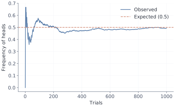

The frequency lurches around early on, then closes in on the expected 0.5 as the tosses pile up.

Throwing dice

The same idea, this time with a variable that isn’t just 0 or 1. A frequency is itself an average — of a variable worth 1 when the event happens and 0 otherwise — so the coin example is a special case. Let’s instead track the running mean of the face values, which should approach the expected value of a fair die, $(1 + 2 + \dots + 6)/6 = 3.5$:

np.random.seed(51)

# 1,000 dice throws, each 1 to 6
dice = np.random.randint(1, 7, 1000)

# Running mean of the face values
dice_mean = [np.mean(dice[:i + 1]) for i in range(len(dice))]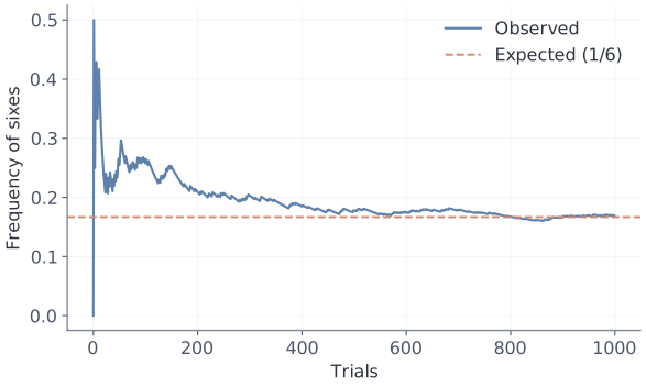

A common confusion

Sometimes you will hear that the law of large numbers means the counts of heads and tails grow closer together as the number of trials increases. That is not what it says — and we can show it. Here is the running difference between the number of heads and the number of tails:

np.random.seed(51)
coin = np.random.randint(0, 2, 1000)

# Cumulative (number of heads) minus (number of tails)
diff = [2 * np.sum(coin[:i + 1]) - (i + 1) for i in range(len(coin))]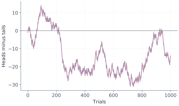

And it isn’t just that our sample happens to look unsettled: the difference is a simple random walk, which converges to nothing — its typical distance from zero grows like $\sqrt{n}$ as trials accumulate.¹ The average converges even as the raw count gap tends to grow. A related mistake is to imagine the coin has some kind of memory, so that a long run of tails makes heads more likely; that is the gambler’s fallacy.

Mathematical treatment

Convergence in probability

A sequence of random variables $X_1, X_2, \dots$ converges in probability to $b$ if, for every $\epsilon > 0$,²

also written

Now let $X_1, X_2, \dots$ be independent and identically distributed (i.i.d.) random variables with expected value $E(X_i) = \mu$, and let $\bar{X}_n = \frac{1}{n}(X_1 + \dots + X_n)$ be the average of the first $n$ of them. The law of large numbers states that this sample average converges in probability to the expected value:³

as $n \to \infty$. This is the weak law of large numbers. Convergence in probability is just one of the ways to define the convergence of a sequence of random variables.⁴ The strong law of large numbers makes a stronger claim — the sample average converges almost surely to the expected value³ — and its proof is beyond our scope here; Terence Tao has a nice exposition on his blog.⁵

Proof of the weak law

Assume additionally that every $X_i$ has finite variance $V(X_i) = \sigma^2$. This assumption is a convenience of the proof below, not a requirement of the law itself, which holds whenever the mean is finite.³ Since the samples are i.i.d.,

and we know that

Chebyshev’s inequality states that, for any random variable $Y$ with finite mean and variance and any $\epsilon > 0$,²

Applying it to $\bar{X}_n$, whose mean is $\mu$ and whose variance is $\sigma^2/n$,

Taking the complement,

As $n \to \infty$ the right-hand side goes to 1, and since a probability can never exceed 1, the left-hand side is squeezed to 1 as well, which gives

The proof also explains the shape of the simulations. The variance of the average shrinks as $\sigma^2/n$, so its typical deviation from $\mu$ shrinks like $1/\sqrt{n}$ — the large early swings and slow final narrowing in the coin and dice plots are exactly this rate at work.